[논문] Modeling Tabular Data using Conditional GAN

Synthetic data

GAN

Author

김보람

Published

March 31, 2023

ref

Introduction

- tabular data GAN

likelihood fitness, machine learning efficiency

- CTGAN

Conditional GANs for synthetic data generation
A benchmarking system for synthetic data geration algorithms

Challenges with GANs in Tabular Data Generation Task

$N_c$: continuous columns $({C_1, \dots, C_{N_c}})$
$N_d$:discrete columns $({D_1, \dots, D_{N_d}})$
위 두개는 각각 $random \ variable$이고 아래와 같이 두 변수의 결합분포를 가진다.
$r_j=(c_{1,j},\dots,c_{N_{c,j}},d_{1,j},\dots,d_{N_{d,j}}), \ j \in {1,\dots,n}$
table $T$ 는 $N_c, N_d$를 포함한다.
data synthesizer $G$를 사용하여 synthetic table $T_{syn}$을 만든다.
$T$ is partitioned into training set $T_{train}$ and test set $T_{test}$.

- $T_{syn}$ 효율성 평가 방법

Likelihood fitness : Do columns in Tsyn follow the same joint distribution as Ttrain?

$T_{syn}$의 columns이 $T_{train}$의 결합분포를 따르는가?

Machine learning efficacy : When training a classifier or a regressor to predict one column using other columns as features, can such classifier or regressor learned from Tsyn achieve a similar performance on Ttest, as a model learned on Ttrain?

- Mixed data types

tabula data는 혼합된 경우가 많다.
이산형 연속형..
GAN은 softmax와 tanh를 사용해야 한다.

- Non-Gaussian distributions

가우시안 분포를 따르는 것은 min-max transformation을 사용해 [-1,1]로 표준화 한다.
연속형 변수는 비가우시안 분포를 사용?

- Multimodal distributions

- Learning from sparse one-hot-encoded vectors

synthetic sample은 softmax를 사용하여 생성한다.
real data는 one-hot vector를 이용한다.

- Highly imbalanced categorical columns

CTGAN Model

- mode-specific normalization을 사용하여 non-Gaussian과 multimodal distribution를 해결한다.

- contidional generator, training-by-sampling 를 통해 불균형이산형(imbalanced discrete columns) 열들을 해결한다.

Notations

– $x_1 \oplus x_2 \oplus \dots$: concatenate vectors $x_1, x_2, \dots$

– $gumbel_{\gamma} (x)$: apply Gumbel softmax with parameter $\gamma$ on a vector $x$

– $leaky_{\gamma}(x)$: apply a leaky ReLU activation on $x$ with leaky ratio $\gamma$

– $FC_{u \to v}(x)$: apply a linear transformation on a $u$-dim input to get a $v$-dim output.

이 외에도 tanh, ReLU, softmax, BN, drop 등을 사용한다.

Mode-specific Normalization

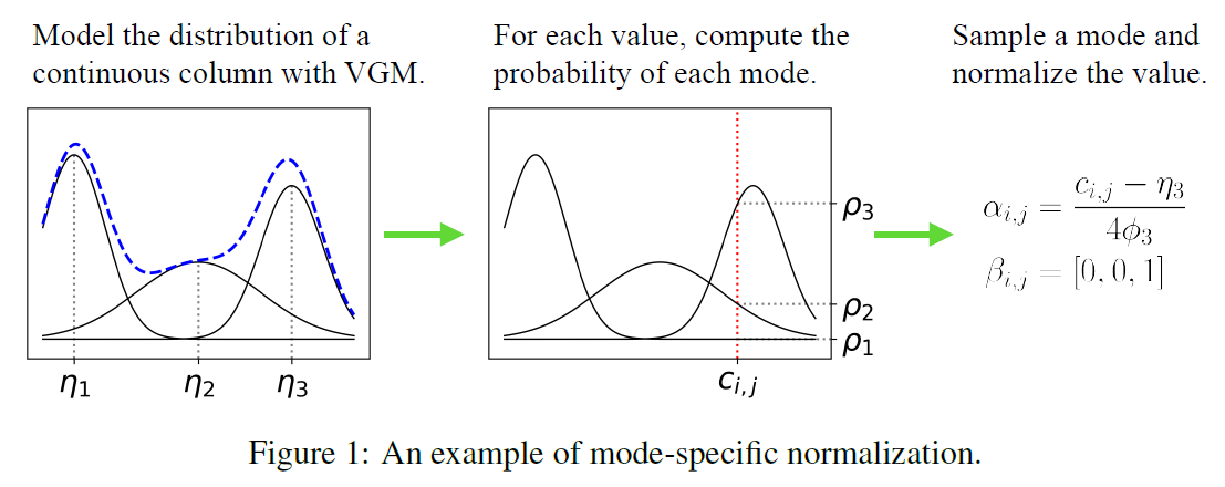
연속형 변수 $C_i$는 variational Gaussian mixture model(VGM) 을 사용한다.

위 예시에서 VGM은 $\eta_1,\eta_2,\eta_3$인 $m_i=3$인 mode를 찾는다.

Gaussian mixture = $\mathbb{P}_{C_i}(c_{i,j}) = \sum_{k=1}^3 \mu_k N (c_{i,j}: \eta_k, \phi_k)$

$\mu_k, \phi_k$ 의 가중치와 분산은 각각 구해놓는다.

$c_{i,j}$의 확률밀도함수는 각각 $\rho_1, \rho_2, \rho_3$이다.

s.t $\rho_k = \mu_k N(c_{i,j}: \eta_k, \phi_k)$

3번째 mode를 선택한다. 원핫인코딩을 통해서 $c_{i,j} \to \beta_{i,j}=[0,0,1]$로 바꾼다.

그리고 $\alpha_{i,j}= \dfrac{c_{i,j}0 - \eta_3}{4\phi_3}$ 가중치를 곱한다.

연속형과 이산형 열들을 바꿔준다.

$r_j = \alpha_{1,j}\oplus \beta_{1,j}\oplus \dots \oplus \alpha_{N_{c,j}} \oplus \beta_{N_{c,j}} \oplus d_{1,j} \oplus \dots \oplus d_{N_{d,j}}$

Conditional Generator and Training-by-Sampling

class imbalance

만약 훈련 데이터가 랜덤샘플에서 훈련된다면 열은 적은카테고리를 가지고 있는 분류를 충분히 대표할수 없다.

이 문제를 the conditional vector, the generator loss, the training-by-sampling method를 이용해 해결하자.

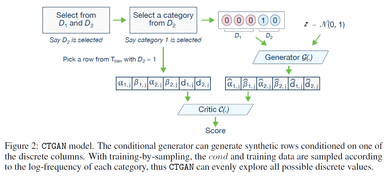
Conditional vector

이산형 분포인 $D_{N_d}$를 원핫인코딩을 통해 $d_{N_d}$로 바꾼다.

For instance, for two discrete columns,D1 = f1, 2, 3g and D2 = f1, 2g,the condition (D2 = 1) is expressed by the mask vectors m1 = [0, 0, 0] and m2 = [1, 0]; so cond = [0, 0, 0, 1, 0].

Generator loss

Training-by-sampling

- Figure2

$m_i^{(k)} = I(if i=i^* \ and \ k=k^*)$

$D_2$ 열을 선택한다. 즉 $i^*=2$이다.
$D_2$에서 첫번째를 선택한다. 즉 $k^*=1$이다.
$m_1=[0,0,0], m_2=[1,0], cond=[0,0,0,1,0]$

Network Structure

generator $\mathbb{g}(z,cond)$

$h_0 = z \oplus cond$
$h_1 = h_0 \oplus ReLU(BN(FC_{|cond|+|z| \to 256}(h_0)))$
$h_2 = h_1 \oplus ReLU(BN(FC_{|cond|+|z|+256 \to 256}(h_1)))$
$\widehat \alpha_i = tanh(FC_{|cond|+|z|+512 \to 1}(h_2)), \ 1 \leq i \leq N_c$
$\widehat \beta_i = gumbel_{0.2}(FC_{|cond|+|z|+512 \to m_i} (h_2)), \ 1 \leq i \leq N_c$
$\widehat d_i = gumbel_{0.2}(FC_{|cond|+|z|+512 \to |D_i|}(h_2)), \ 1 \leq i \leq N_c$

critic $C(r_1,\dots,r_{10},cond_1,\dots,cond_{10})$

- use PacGAN with 10 samples in each pac to prevent mode collapse

$h_0 = r_1 \oplus \dots \oplus r_{10} \oplus cond_1 \oplus \dots \oplus cond_{10}$
$h_1 = drop(leaky_{0.2}(FC_{10|r|+10|cond| \to 256}(h_0)))$
$h_2 = drop(leaky_{0.2}(FC_{256 \to 256}(h_1)))$
$C(\cdot) = FC_{256 \to 1}(h_2)$

Adam optimaizer 사용한 학습률 $2·10^{-4}$

TVAE Model

- TVAE generator

$h_1 = ReLU(FC_{128 \to 128}(z_j))$
$h_2 = ReLU(FC_{128 \to 128}(h_1))$
$\bar \alpha _{i,j} = tanh(FC_{128 \to 1}(h_2)) \ , \ 1 \leq i \leq N_c$
$\widehat \alpha_{i,j} \sim N(\bar \alpha_{i,j} , \delta_i) \ , \ 1 \leq i \leq N_c$
$\widehat \beta_{i,j} \sim softmax(FC_{128 \to m_i} (h_2)) \ , \ 1 \leq i \leq N_c$
$\widehat d_{i,j} \sim softmax(FC_{128 \to |D_i|}(h_2)) \ , \ 1 \leq i \leq N_d$
$p_\theta(r_j|z_j) = \Pi_{i=1}^{N_c} \mathbb{P}(\widehat \alpha_{i,j} = \alpha_{i,j}) \Pi_{i=1}^{N_c} \mathbb{P}(\widehat \beta_{i,j} = \beta_{i,j}) \Pi_{i=1}^{N_d} \mathbb{P}(\widehat \alpha_{i,j} = \alpha_{i,j})$

$\widehat \alpha_{i,j}, \widehat \beta_{i,j}, \widehat d_{i,j}$ : random variable

$p_\theta(r_j|z_j)$ : joint distribuion

TVAE를 Adam으로 학습한 학습률: $1e^{-3}$

Benchmarking Synthetic Data Generation Algorithms

Baselines and Datasets

simulated data

오라클 S로부터 $T_{train}, T_{test}$을 만든다.
이 오라클은 가우시안 혼합 모델 또는 베이지안 네트워크이다.
GridR:각 모드에 랜덤 오프셋을 추가
베이지안 네트워크: alarm, child, asia, insurance를 사용

real datasets

UCI머신러닝에서 사용되는 6개 사용
adult, census, covertype, intrusion,news
MNIST 사용

Evaluation Metrics and Framework

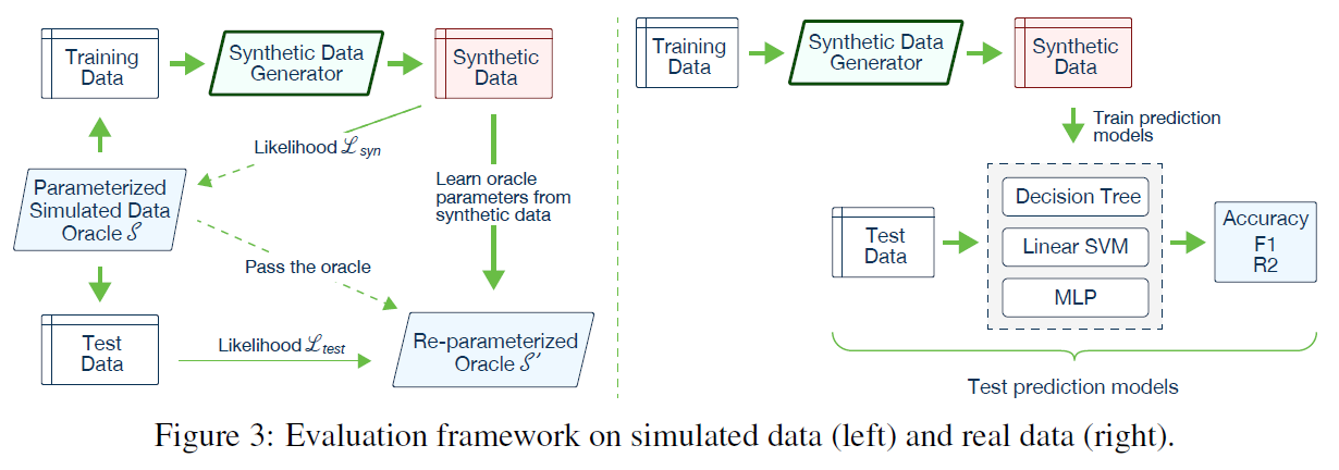
Likelihood fitness metric

simulated data 사용
$T_{syn} L_{syn},T_{test} L_{test}, $
$L_{syn}$이 과적합되는 문제를 해결하기 위하 $L_{test}$를 사용

Machine learning efficacy

real dataset 사용
accruracy와 F1, $\mathbb{R^2}$ 측정

Benchmarking Results

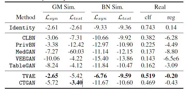
GM Sim : Gaussian mixture
BN Sim : Bayesian networks
TVAE가 CTGAN보다 우수한 편이지만 privacy해결은 못하므로 privacy생각하면 CTGAN사용..

Dataset Details

– Adult: http://archive.ics.uci.edu/ml/datasets/adult

– Census: https://archive.ics.uci.edu/ml/datasets/census+income

– Covertype: https://archive.ics.uci.edu/ml/datasets/covertype

– Credit: https://www.kaggle.com/mlg-ulb/creditcardfraud

– Intrusion: http://archive.ics.uci.edu/ml/datasets/kdd+cup+1999+data

– MNIST: http://yann.lecun.com/exdb/mnist/index.html

– News: https://archive.ics.uci.edu/ml/datasets/online+news+popularity

사용예시

#pip install ctgan

from ctgan import CTGAN
from ctgan import load_demo

real_data = load_demo()

# Names of the columns that are discrete
discrete_columns = [
    'workclass',
    'education',
    'marital-status',
    'occupation',
    'relationship',
    'race',
    'sex',
    'native-country',
    'income'
]

ctgan = CTGAN(epochs=10)
ctgan.fit(real_data, discrete_columns)

# Create synthetic data
synthetic_data = ctgan.sample(1000)

synthetic_data

	age	workclass	fnlwgt	education	education-num	marital-status	occupation	relationship	race	sex	capital-gain	capital-loss	hours-per-week	native-country	income
0	21	Private	168287	HS-grad	14	Married-civ-spouse	Transport-moving	Unmarried	Black	Male	27	2	47	United-States	<=50K
1	40	Local-gov	129105	HS-grad	14	Married-civ-spouse	Machine-op-inspct	Husband	Other	Female	127	1503	40	United-States	<=50K
2	19	State-gov	182904	Some-college	10	Divorced	Adm-clerical	Wife	White	Male	-17	-4	40	United-States	<=50K
3	34	Self-emp-inc	203270	1st-4th	1	Never-married	Prof-specialty	Not-in-family	White	Male	121	1918	29	United-States	<=50K
4	23	Private	181278	10th	3	Never-married	?	Husband	White	Male	8805	6	38	China	<=50K
...	...	...	...	...	...	...	...	...	...	...	...	...	...	...	...
995	28	State-gov	29365	Some-college	5	Married-civ-spouse	Adm-clerical	Husband	Asian-Pac-Islander	Male	16	-6	40	United-States	>50K
996	27	Private	130995	HS-grad	1	Married-civ-spouse	Exec-managerial	Husband	White	Female	35	2	49	Canada	<=50K
997	35	Private	128850	Some-college	3	Married-spouse-absent	Adm-clerical	Unmarried	White	Female	119	-7	40	United-States	<=50K
998	28	Private	188708	HS-grad	10	Married-spouse-absent	Prof-specialty	Not-in-family	Black	Male	58	-1	40	United-States	<=50K
999	30	Private	146128	Some-college	2	Married-civ-spouse	Sales	Husband	White	Female	85	0	26	United-States	<=50K

1000 rows × 15 columns

[논문] Modeling Tabular Data using Conditional GAN

ref

Introduction

Challenges with GANs in Tabular Data Generation Task

CTGAN Model

Notations

Mode-specific Normalization

Conditional Generator and Training-by-Sampling

Conditional vector

Generator loss

Training-by-sampling

Network Structure

generator \(\mathbb{g}(z,cond)\)

critic \(C(r_1,\dots,r_{10},cond_1,\dots,cond_{10})\)

TVAE Model

Benchmarking Synthetic Data Generation Algorithms

Baselines and Datasets

simulated data

real datasets

Evaluation Metrics and Framework

Likelihood fitness metric

Machine learning efficacy

Benchmarking Results

Dataset Details

사용예시

ref

Introduction

Related Work

Challenges with GANs in Tabular Data Generation Task

CTGAN Model

Notations

Mode-specific Normalization

Conditional Generator and Training-by-Sampling

Conditional vector

Generator loss

Training-by-sampling

Network Structure

generator \(\mathbb{g}(z,cond)\)

critic \(C(r_1,\dots,r_{10},cond_1,\dots,cond_{10})\)

TVAE Model

Benchmarking Synthetic Data Generation Algorithms

Baselines and Datasets

simulated data

real datasets

Evaluation Metrics and Framework

Likelihood fitness metric

Machine learning efficacy

Benchmarking Results

Dataset Details

사용예시